Tutorials Level 0
Preparing the input cube
Make sure your cube :
- is written as a fits file
- has a third dimension representing wavelengths or frequencies.
- has a minimum info in the header.
- The header should have units but the algorithm works in velocity space (dlamba/lamba or dfrequency/frequency). Check the Instrument.z_step_kms value which is critial for the kinematic parameters.
- If the header is incomplete (CRPIX3, CDELT3, CRVAL3, CUNIT3), the algorithm will try to use the default values assigned to the instrument. The user can specify these directly.
- is adequately cropped in x and y and along z around the galaxy (performance goes as Npix log(Npix)!)
- is continuum subtracted (!) as the algorithm does not fit the continuum
- best to provide the variance in a separate file or via a MPDAF
Obj.Cube. If no variance is specified, the cube statistics will be used.
Warning
You should specify the PSF and spectral LSF that are in effect for your cube. Don’t trust the defaults.
Note
For MPDAF users, a MPDAF Obj.Cube object is ok as input.
Test GalpaK with MUSE per default
The simplest way to use GalPaK is as follows :
import galpak
gk = galpak.run('GalPaK_cube_1101_from_paper.fits', seeing=1.0, instrument=galpak.MUSEWFM())
or if you want to auto-tune the random_scale parameter:
import galpak
gk = galpak.autorun('GalPaK_cube_1101_from_paper.fits', seeing=1.0, instrument=galpak.MUSEWFM())
where seeing is the PSF’ FWHM which is short for :
import galpak
gk = galpak.GalPaK3D('GalPaK_cube_1101_from_paper.fits', seeing=1.0, instrument=galpak.MUSEWFM())
gk.run_mcmc()
Warning
seeing=1.0 is equivalent to galpak.MUSE(psf_fwhm=1.0) The proper way to specify the seeing is specified in customizing-the-psf.
The input can also be a Hyperspectral Cube.
Actually, GalPaK will instantiate one from your fits file if you pass a string filename.
Note
You can find other test FITS cubes in data/input/.
- The cube_1101 input parameters are:
xo yo zo radius incl PA rv Vmax flux Sig_o GaussianFWHM
15.0 15.0 15.0 4.0841 60.0 50.0 1.35 199.5 1e-16 80.0 1.0
The gk.galaxy parameters from the run above should be close to this:
Galaxy Parameters : value (± stdev) [units]     [Confidence Interval]
   x: 15.06 ± 0.08 (pixel)      CI 95%: [14.90,15.19]
   y: 15.05 ± 0.07 (pixel)      CI 95%: [14.91,15.20]
   z: 15.055705 ± 0.056999 (pixel)      CI 95%: [14.948377,15.164004]
   flux: 8.41e-17 ± 2.07e-18 (same units as the input Cube)     CI 95%: [8.14e-17,8.86e-17]
   radius: 4.10 ± 0.16 (pixel)  CI 95%: [3.76,4.41]
   inclination: 69.74 ± 2.07 (deg)      CI 95%: [66.64,73.99]
   pa: 125.83 ± 1.99 (deg)      CI 95%: [121.37,129.05]
   turnover_radius: 1.37 ± 0.27 (pixel)         CI 95%: [1.09,2.11]
   maximum_velocity: 202.74 ± 13.21 (km/s)      CI 95%: [183.77,236.45]
   velocity_dispersion: 81.05 ± 4.68 (km/s)     CI 95%: [72.97,93.14]
Warning
The cube has units `erg/s/cm2/AA’, so the galaxy flux is 8.4e-17 erg/s/cm2/AA * 1.25 Angstrom = 1.05e-16 erg/s/cm2. The flux is thus:
gk.galaxy.flux * gk.cube.z_step
Test galpak with your cube
Assuming your cube has units of Angstrom (default for MUSE) :
from galpak import GalPaK3D
gk = GalPaK3D('GalPaK_cube_1101_from_paper.fits', seeing=1.0, instrument=galpak.MUSE(lsf_fwhm=2.51))
For MPDAF users, a MPDAF Obj.Cube object is ok as input, which handles the variance :
from mpdaf import obj
objcube = obj.Cube('GalPaK_cube_1101_from_paper.fits')
gk = GalPaK3D(objcube, seeing=1.0, instrument=galpak.MUSE(lsf_fwhm=2.51))
Note
Currently, the variance can also be specified manually :
gk = GalPaK3D('my_cube.fits',variance='my_variance.fits', seeing=1.0, instrument=galpak.MUSE(lsf_fwhm=2.51))
In future version, the variance can be specified as a “STAT” or “VARIANCE” extension to the fits file.
Run galpak examples
Assuming your cube can be read properly, you can run it with :
from galpak import GalPaK3D
gk = GalPaK3D('GalPaK_cube_1101_from_paper.fits', seeing=1.0, instrument=galpak.MUSE(lsf_fwhm=2.51))
gk.run_mcmc(max_iteration=500)
gk.save('my_galpak_run')
or with the api :
import galpak
my_instrument = galpak.MUSE(lsf_fwhm=2.51)
gk = galpak.run('galpak_125_seeing1.0_flux1e-16.fits', seeing=1.0, instrument=my_instrument, max_iterations=500)
gk.save('my_galpak_run')
Typically you will need 5000 or 10000 iterations
Warning
Make sure to look at the MCMC chain. Have all the parameters converged?
A practical example
Initialize with :
gk = GalPaK3D(my_file, seeing=0.8,instrument=galpak.SINFOJ250())
- or
- gk = GalPaK3D(my_file, seeing=0.8,instrument=galpak.ALMA())
Check the instrument properties with :
print gk.instrument
Check that it has the central wavelength z_central taken from the fits header,
which determines the right velocity ‘step’ (cdelt3 in km/s). If the header is not correct, you have
several options to set the central wavelength with z_central or cdelt3 or cunit3.
Check that the LSF and PSF parameters are ok - see below for how to tweak them.
Run with :
gk.run_mcmc()
Save everything with :
gk.save('my_output')
and check again that the 3D kernel gk.psf3d is correct !
A wrong kernel will lead to unphysical results.
Default Model Parameters
Both run and run_mcmc use a DiskModel object with exponential flux profile per default,
arctangent rotation profile and thick disk dispersion.
You can see the detailed documentation for the available parameters from the model class,
but here’s a highlight of the most important ones :
flux_profile: ‘gaussian’ or ‘exponential’ [default] or ‘de_vaucouleurs’The flux profile of the galaxy.
rotation_curve: The profile of the velocity v(r) can be in- ‘isothermal’ : a pseudo-isothermal V~Vmax (1-actan(X)/X) where X=r/rV, rV=turnover_radius
- ‘arctan’ (default) : V~ Vmax arctan(r/rV), rV=turnover radius
- ‘tanh’ : an tanh profile V~Vmax tanh(r/rV)
- ‘exp’ : inverted exponential, 1-exp(-r/rV)
- ‘mass’ : a constant light-to-mass ratio v_circ(r)=sqrt(G m(<r) / r)
disk_dispersion: ‘thick’ or ‘thin’ (or ‘infinitely_thin’ TBD)The local disk dispersion from the rotation curve and disk thickness from Binney & Tremaine 2008 see Cresci et al. 2007, Genzel et al. 2008 for details. GalPak has 3 components for the dispersion:
- a component from the rotation curve arising from mixing velocities of a disk with non-zero thickness
- a component from the local disk dispersion specified by
run_mcmc.disk_dispersion - a spatially constant dispersion, [which is the output parameter
gk.galaxy.velocity_dispersion]
Warning
From v1.9.0, you should change these options in ``run_mcmc’’ as follows :
mydisk = galpak.DiskModel(flux_profile=’gaussian’, rotation_curve=’isothermal’)
or using the API run_ or autorun_ method:
import galpak
my_instrument = galpak.MUSE(lsf_fwhm=2.51)
mydisk = galpak.DiskModel(flux_profile='gaussian', rotation_curve='isothermal')
gk = galpak.run('galpak_125_seeing1.0_flux1e-16.fits', seeing=1.0, instrument=my_instrument, model=mydisk, max_itrations=500)
gk.save('my_galpak_run')
You can always check your model with :
print(gk.model)
Run Output Overview
The run_mcmc method returns a GalaxyParameters object.
Type :
print gk.galaxy
to see the parameters (gk.error contains the error vector).
Use the methods of GalaxyParameters tofile or tolist
to store this.
The run_mcmc also fills the gk instance parameters with several output data :
gk.deconvolved_cube: best guess as to what the deconvolved cube should begk.convolved_cube: virtually convolved cube, should be close to the inputted measure cubegk.residuals_cube: differential between measure cube and convolved cube, inversely scaled by measure errorgk.psf3d: the 3D PSF*LSF used for the convolutiongk.chain: the full markov chain, with each step holding its galaxy parameters and reduced χgk.acceptance_rate: the final proportion of useful iterations in%gk.initial_parameters: the first parameters of the markov chaingk.galaxy: a view to the returnedGalaxyParametersobjectgk.error: the error margin of above galaxy parametersgk.true_flux_map: the intrinsic flux mapgk.true_velocity_map: the intrinsic velocity fieldgk.true_disp_map: the intrinsic dispersion map
Save the run
Once the MCMC has run, you can save the results to file easily :
import galpak
gk = galpak.run('my_cube.fits',instrument=galpak.MUSEWFM())
gk.save('my_run')
It will create a bunch of files prefixed by my_run in the current working directory.
See the save() method documentation for the list of files that will be created.
Tutorials Level 1
MCMC chain tuning
Again, you can see the detailed documentation for the available parameters,
but the most important parameters to tune are :
random_scale: a scale factor to the width of the proposal distribution (Cauchy). A good practice is to tune this to have an acceptance rate of 30-50 %. (for example, the valuerandom_scale=2sets a factor 2x from the defaults)max_iterations: max number of (accepted) iterations [default=10000]method: ‘last’ or ‘chi_sorted’ or ‘chi_min’- Method used to determine the best parameters from the chain.
- ‘last’ (default) : mean of the last_chain_fraction(%) last parameters of the chain
- ‘chi_sorted’ : mean of the last_chain_fraction(%) best fit parameters of the chain
- ‘chi_min’ : mean of last_chain_fraction(%) of the chain around the min chi
last_chain_fraction: last fraction of chain (in %) to use to determine the best parameters [default=60]min_acceptance_rate: minimum acceptance rate (in %) to keep going. [default: 5]
Using Custom Boundaries
You can make sure that GalPaK will not try to find galaxy parameters outside of explicit boundaries :
from galpak import run, GalaxyParameters
min_boundaries = GalaxyParameters(x=5.)
max_boundaries = GalaxyParameters(x=7., y=9.)
gk = run('my_muse_cube.fits',
         min_boundaries=min_boundaries,
         max_boundaries=max_boundaries)
The boundaries you provide will be merged into the default boundaries.
Note
For Vmax ‘maximum_velocity’, the min and max boundaires should be equal, e.g [-300,300]
Tweaking the Random Walk
You can (and should) tweak the random_scale parameter of the run_mcmc method
in order to get an acceptance rate around 30-40 %.
The value you provide is the a coefficient (default=1)
applied to the random walk of the parameters.
A bad chain, poorly scaled
But when you provide a random_scale with values greater than 1, say 5 :
from galpak import GalPaK3D
glpk3d = GalPaK3D('my_muse_cube.fits')
galaxy = glpk3d.run_mcmc(random_scale=5.)
… you get a more excited chain :

A good chain with a more thorough walk
Conversely, a less-than-one random_scale, in combination with initial_parameters,
can be used to fine-tune your results by reducing the steps of the random walk.
Also, you can tweak the random walk of only a subset of the parameters by passing a GalaxyParameters object :
galaxy = glpk3d.run_mcmc(random_scale=GalaxyParameters(x=10., pa=2.))
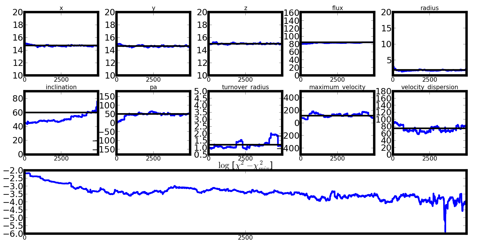
Plotting the Markov chain
Once a deconvolution has been computed, you can plot the Markov chain that was created :
from galpak import GalPaK3D
glpk3d = GalPaK3D('GalPaK_cube_1101_from_paper.fits', seeing=1.0, instrument=galpak.MUSE(lsf_fwhm=2.51))
galaxy = glpk3d.run_mcmc(max_iterations=15e3)

# Show plot on-screen
galpak.plot_mcmc()

# Save plot to png or jpg file
galpak.plot_mcmc(filepath='my_mcmc_plot.png')
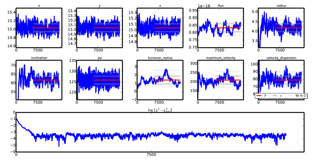
An example of chain plotting for the GalPaK_cube_1101_from_paper.fits with N=15,000 iterations
Plotting the cross-correlations
After a galpak run has been completed, you can plot the correlations in the Markov chain with :
from galpak import GalPaK3D
glpk3d = GalPaK3D('GalPaK_cube_1101_from_paper.fits', seeing=1.0, instrument=galpak.MUSE(lsf_fwhm=2.51))
galaxy = glpk3d.run_mcmc(max_iterations=15e3)

# Show plot on-screen
galpak.plot_correlations()

# Save plot to png or jpg file
galpak.plot_correlations(filepath='my_correlations.png')
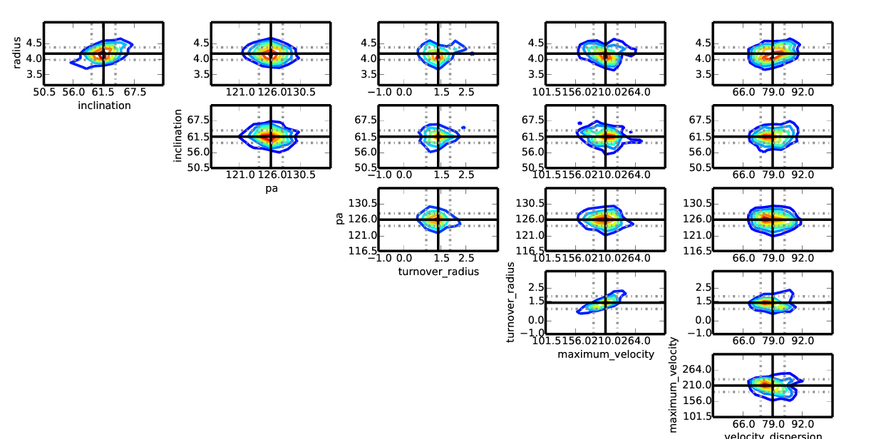
An example of chain plotting for the GalPaK_cube_1101_from_paper.fits with N=15,000 iterations
Plotting the cubes’ images
Once a deconvolution has been computed, you can plot the resulting cubes :
from galpak import GalPaK3D
glpk3d = GalPaK3D('my_muse_cube.fits')
galaxy = glpk3d.run_mcmc()

# Show plot on-screen
galpak.plot_images()

# Save plot to png or jpg file
galpak.plot_images(filepath='my_plot.png')

# Crop the rendered cubes along z, around the galaxy's z
galpak.plot_images(z_crop=7)
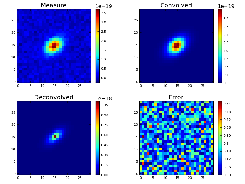
An example of images plotting
Recover the parameters from an earlier save
Once you’ve saved the run to disk, you can use the following from_file method to read the parameters:
params = GalPaK3D.GalaxyParameters()
params.from_file('my_param_file.dat')
Recover the chain from an earlier save
Once you’ve saved the run to disk, you can use the following snippet to re-iterate through the chain:
import asciitable
with open('my_run_chain.dat', 'r') as chain_file:
    data = asciitable.read(chain_file.read(), Reader=asciitable.FixedWidth)
for data_record in data:
    # <your logic here>
    print(data_record.x)
    print(data_record.reduced_chi)
or simpy using the import_chain method:
glpk3d = GalPaK3D('my_muse_cube.fits')
glpk3d.import_chain('my_chain.dat')
Cubes from another instrument
You can specify the instrument that will convolve the simulated data.
import galpak
gk = galpak.run('my_musenfm_cube.fits', instrument=galpak.MUSENFM())
Instruments accept two parameters: psf and lsf :
from galpak import run, MUSENFM, GaussianPointSpreadFunction, GaussianLineSpreadFunction
my_psf = GaussianPointSpreadFunction(fwhm=1.2, pa=0., ba=1.0)
my_lsf = GaussianLineSpreadFunction(fwhm=0.00065)
gk = run('my_musenfm_cube.fits', instrument=MUSENFM(psf=my_psf, lsf=my_lsf))
By default, the instrument will combine the psf (2D) and the lsf (1D) into a 3D spread function
and will apply it to the cube in the method convolve(cube).
Tutorials Level 2
Setting a parameter to a fixed value
You can use the parameter known_parameter, which takes a GalaxyParameters as in the example here:
import galpak
fixed = galpak.GalaxyParameters().copy()
fixed.turnover_radius = 1
gk = GalPaK3D('GalPaK_cube_1101_from_paper.fits', seeing=1.0, instrument=galpak.MUSE(lsf_fwhm=2.51))
gk.run_mcmc(max_iteration=500,known_parameters=fixed)
Using line doublets
You can use the parameter line, a dictionary, to tell galpak you’re expecting a dual peak :
from galpak import GalPaK3D
glpk3d = GalPaK3D('my_muse_cube.fits', line={'wave': [3726.2, 3728.9], 'ratio': [0.8, 1.0]})
galaxy = glpk3d.run_mcmc()
or using the API :
from galpak import GalPaK3D
res = GalPaK3D.run('my_muse_cube.fits', line={'wave': [3726.2, 3728.9], 'ratio': [0.8, 1.0]})
Note
Only the rest-wavelengths are needed regardless of redshift because the algorithm works in velocity space. Here, you specify the velocity difference for the two lines in the doublet, 3e5*(l2-l1)/(l1+l2)*2, so the redshift does not matter.
Warning
For version >= 1.9.0, this line parameter is now part of the DiskModel class.
So for GalPaK3D v1.9.0 and beyond, the line should be used as :
from galpak import GalPaK3D, DiskModel
myline = {'wave': [3726.2, 3728.9], 'ratio': [0.8, 1.0]}
glpk3d = GalPaK3D('my_muse_cube.fits')
galaxy = glpk3d.run_mcmc(model=DiskModel(line=myline))
or using the API
from galpak import GalPaK3D, DiskModel
myline = {'wave': [3726.2, 3728.9], 'ratio': [0.8, 1.0]}
disk = DiskModel(line=myline)
res = GalPaK3D.run('my_muse_cube.fits', model=disk )
Note
For version = 1.9.0, this line parameter can also be used as in prior versions.
Customizing the Point Spread Function
Tweaking the PSF
You can either specify the seeing parameter as in the example above, or change its attributes from the Instrument parameters :
from galpak import GalPaK3D, SINFOK250, GaussianPointSpreadFunction

# this one-liner
my_instrument = SINFOK250(psf=GaussianPointSpreadFunction(fwhm=0.7,pa=0.1,ba=0.9))

# is equivalent to
my_instrument = SINFOK250()
my_instrument.psf.fwhm = 1.5
my_instrument.psf.pa = 0.1
my_instrument.psf.ba = 0.9

# and, as the gaussian PSF is the default, you can also fast-tweak it this way
my_instrument = SINFOK250(psf_fwhm=0.7, pa=0.1, ba=0.9)

# then, whatever way you used to create your instrument, use it like this
glpk3d = GalPaK3D('my_sinfok250_cube.fits', instrument=my_instrument)
galaxy = glpk3d.run_mcmc()
De-activating the PSF
You can de-activate the PSF entirely :
from galpak import GalPaK3D, SINFOK250, NoPointSpreadFunction

glpk3d = GalPaK3D('my_sinfok250_cube.fits', instrument=SINFOK250())
glpk3d.instrument.psf = None
galaxy = glpk3d.run_mcmc()

# ... is the same as
glpk3d = GalPaK3D('my_sinfok250_cube.fits', instrument=SINFOK250())
glpk3d.instrument.psf = NoPointSpreadFunction()
galaxy = glpk3d.run_mcmc()
Using another PSF
You can specify another PSF you want to use with the instrument :
from galpak import GalPaK3D, SINFOK250, MoffatPointSpreadFunction

glpk3d = GalPaK3D('my_sinfok250_cube.fits', instrument=SINFOK250())
glpk3d.instrument.psf = MoffatPointSpreadFunction(
    alpha=1.11,  # (uninformed/dummy example value)
    beta=2.22    # (uninformed/dummy example value)
)
The galpak module provides GaussianPointSpreadFunction and
MoffatPointSpreadFunction.
They each have a number of parameters you may provide upon instantiation.
If you don’t, default values inferred from the Instrument and Cube will be used :
glpk3d = GalPaK3D('my_muse_cube.fits')
print glpk3d.instrument.psf

# psf = Gaussian PSF :
#   fwhm         = 0.8 "
#   pa           = 0 °
#   ba           = 1.0
Using custom image for the PSF
You can specify an empirically determined PSF (e.g. from a bright star) using
the class ImagePointSpreadFunction
which accepts fits file or ndarray :
import galpak
my_psf = galpak.ImagePointSpreadFunction('my_psf_image.fits')
gk = galpak.GalPak3D('my_cube.fits', instrument=galpak.MUSEWFM())
gk.instrument.psf = my_psf
print gk.instrument

#psf = Custom Image PSF
#lsf = Gaussian LSF : fwhm = 2.675  Angstrom
or :
import galpak, pyfits
image_array = pyfits.open('my_psf_image.fits')[0].data
instrum = galpak.MUSEWFM(psf=galpak.ImagePointSpreadFunction(image_array) )
gk = galpak.GalPak3D('my_cube.fits', instrument=instrum)
print gk.instrument

#psf = Custom Image PSF
#lsf = Gaussian LSF : fwhm = 2.675  Angstrom
Warning
The custom PSF image must be well centered, otherwise the centroid positions will be off. Ideally, (xo, yo) should be :
xo = (shape[1] - 1) / 2 - (shape[1] % 2 - 1)
yo = (shape[0] - 1) / 2 - (shape[0] % 2 - 1)
where shape is the image shape (which should be the same shape as the cube.shape[1:] spatial dimensions).
Making your own PSF
You can create your own PSF, it just needs to implement PointSpreadFunction.
A good example of this is the NoPointSpreadFunction class :
from galpak import PointSpreadFunction


class NoPointSpreadFunction(PointSpreadFunction):
    """
    A spread function that does not spread anything, and will leave the cube unchanged.
    Passing this class to the instrument's psf is the same as passing None.
    """
    def __init__(self):
        pass

    def as_image(self, for_cube):
        """
        Return the identity PSF, chock-full of zeros.
        """
        # Here, you may create your own 2D PSF image and then return it
        shape = for_cube.shape[1:]
        return np.zeros(shape)
Customizing the Line Spread Function
Using another LSF
You can specify another LSF you want to use with the instrument :
glpk3d = GalPaK3D('my_muse_cube.fits', instrument=MUSEWFM(lsf=MUSELineSpreadFunction()))
The galpak module provides GaussianLineSpreadFunction and
MUSELineSpreadFunction.
They each have a number of parameters you may provide upon instantiation.
Making your own LSF
You can create your own LSF, it just needs to implement LineSpreadFunction.
Creating a custom instrument
You can also create your own instrument, by extending galpak.Instrument.
You can override the calibrate and convolve methods :
from galpak import Instrument


class MyInstrument(Instrument):

    # This callback is called by GalPaK3D during its init
    def calibrate(self, cube):
        """
        The cube is a HyperspectralCube, and
        it has additional attributes provided by GalPaK3D :
            - xy_step (in ")
            - z_step (in µm)
            - z_central (in µm)
        """
        # <Your logic here>
        # Important : run the default calibration in the end
        Instrument.calibrate(self, cube)

    # Optionally, you may override the convolution method
    # By default it applies the PSF3D, see Instrument implementation
    def convolve(self, cube):
        """
        Convolve the provided data cube.
        Should transform the input cube and return it, it is faster than copying.
        """
        # <convolve the cube>
        return cube
Note
If you do create your own instrument, please consider making a pull request !
Adding another Galaxy Parameter
Note
This is for advanced users only.
The file you want to edit is lib/galaxy_parameters.py.
Say you want to add a new galaxy parameter named sugar :
Update the list
GalaxyParameters.names, add ‘sugar’ at the end.Add the property after the others :
sugar = GalaxyParameter(name='sugar', key=10, doc="Some more sugar", unit="sweetness", precision="3.2f")
Here are the parameters you can provide the describe the new galaxy parameter :
- name (string) : the name of the variable (MUST be the same as the name in
GalaxyParameters.names.) - key (int) : the position in the the ndarray of this parameter
- short (string) : a shorter name, for compact display
- doc (string) : some documentation that will appear to the enduser.
- unit (string) : the unit, if any
- precision (string) : the precision to use during string casting, as used by
string.format().
- name (string) : the name of the variable (MUST be the same as the name in
Update this class’
__init__()method (signature and assignation)Update this class’
__new__()method (signature and call to__init__)
Tutorials Level 3
Reading old parameter file
If you want to read the output parameters from an old run, you can do so:
gk=galpak.GalPak3D(mycube_name,instrument=myinstrument)
gk.galaxy.from_file(prefix+'_galaxy_parameters.dat')
gk.galaxy
If you want to use an array to set parameters (in order to change the boundaries, e.g.), you can do so:
from galpak import GalaxyParameters
gp = GalaxyParameters.from_ndarray(my_ndarray_of_data)
You can also convert the parameters to an astropy.table:
t = gk.galaxy.as_table()
or turn it into a vector ndarray:
v = gk.galaxy.as_vector()
Reading old chain, recomputing parameters
If you want to read an old run and recompute the parameters using a different method or settings:
gk=galpak.GalPak3D(mycube_name,instrument=myinstrument)
gk.import_chain(prefix+'_chain.dat', compute_best_parameters=True)
gk.galaxy
this will use the best_parameters_from_chain method to compute the galaxy parameters, with the parameters (method=’last’, chain_fraction=60, percentile=95).
If you want to customize further:
gk=galpak.GalPak3D(mycube_name,instrument=myinstrument)
gk.import_chain(prefix+'_chain.dat', compute_best_parameters=False)
gk.best_parameters_from_chain(method_chain='last', chain_fraction=40, percentile=68)
gk.galaxy
Handling of parameter names
You can construct a dictionary of shortcut names for each of the parameter:
my_dict = gk.galaxy.short_dict()
Or access each as:
short = gk.galaxy.__shorts__('inclination')
Tutorials Level 4
Changing of chi2 statistics
GalPak3D accepts the following statistics to perform the parameter optimization, which can be set with the parameter `chi_stat’:
- “gaussian” [default] to perform the sum of residual squares (aka. normal chi2), i.e. sum ( D_i - M_i )^2 / stdev_i^2
When the noise in the data is poissonian, the following options are available:
Warning
This is experimental and has not been validated. Please use with caution and send feedback.
- “Neyman” using the Modified Neyman statistic from Humphrey 2009, i.e. Sum ( M_i - D_i )^2 / max(D_i,1)
- “Pearson” using the Pearson statistic Humphrey 2009, i.e. Sum ( M_i - D_i )^2 / M_i
- “Mighell” using the Mighell modified Statistic Mighell 1998, i.e. Sum ( D_i + min(1,D_i) - M_i)^2 / D + 1
- “Cstat” using the Cash-statistic from Cash 1979 described in Humphrey 2009, i.e. Sum ( M_i - D_i + D_i * log(D_i/M_i) )